Climate risk assessment: Charleston County, South Carolina

Results summary

As a result of climate change, flood risk is expected to increase throughout Charleston County. The probability of the 100-year rainfall event, a useful indicator of flood risk, will likely triple by the mid 21st century. The trend shifts slightly back by the end of the century, although the probability of the 100-year rainfall event will still be more than double present day. Sea levels are also projected to rise 0.37 meters (1.21 ft) by 2050 and 0.75 meters (2.46 ft) by 2080. This will translate into greater flood depths and extent for Charleston County. Here we present our findings on extreme precipitation and flooding to help Charleston County in its plans to create a more resilient future for all residents.

Extreme rainfall

The Fourth National Climate Assessment shows that the U.S. Southeast region has seen a 27% increase of annual precipitation falling in the heaviest 1% of events.¹ This trend of intensification is expected to continue under future warming. Intensification here speaks to both more frequency and more severe rainfall events. Here we use localized future precipitation data from a downscaled global climate model to calculate the change in probability of extreme rainfall events. A detailed explanation of the precipitation data processing can be found in the accompanying methodology document. In Figure 1, we show the changes in the return period of the historical (2000–2020) 100-year rainfall event for 2040–2060 and 2070–2090. By 2040–2060 and 2070–2090, the historical 100-year event will occur with a return period between 1-in-20 to 1-in-60 years and 1-in-30 to 1-in-80 years, respectively.

According to the National Atlas 14 published by the National Oceanic and Atmospheric Administration (NOAA), the historical 100-year rainfall amount in Charleston County, SC is 10.3 inches. By 2040–2060, Charleston County’s average 100-year rainfall amount increases to 12.7 inches and by 2070–2090 this decreases to 11.7 inches (Figure 2). Potential reasons for this downward trend in rainfall intensification later in the century include decadal variability or a change in the spread of the model ensemble resulting in a slight shift in extreme rainfall distributions. Nevertheless, the climate change signal is still present as the 100-year event intensifies through the 21st century relative to the 2000–2020 time period.

¹ USGCRP, 2018: Impacts, Risks, and Adaptation in the United States: Fourth National Climate Assessment, Volume II [Reidmiller, D.R., C.W. Avery, D.R. Easterling, K.E. Kunkel, K.L.M. Lewis, T.K. Maycock, and B.C. Stewart (eds.)]. U.S. Global Change Research Program, Washington, DC, USA, 1515 pp. https://doi.org/10.7930/NCA4.2018

Flooding

In addition to the intensification of extreme rainfall events, sea levels are also expected to rise significantly through the 21st century under climate change. According to the IPCC AR6 projections, sea levels will rise 0.37 meters (1.21 ft) by 2050 and 0.75 meters (2.46 ft) by 2080 under the SS5-8.5 Low Confidence scenario (Low Confidence refers to greater Antarctica and Greenland ice sheet melting than the SS5-8.5 Medium Confidence scenario). With increased rainfall amounts and higher sea levels comes greater flood risk. For a detailed explanation of the flood model input data and flood modeling procedures, please refer to the accompanying methodology document.

Flood extent comparison

Before estimating future flood risk, we compare the present-day flood risk results against the Federal Emergency Management Agency (FEMA) flood maps as a validation exercise. FEMA maps are not ground truth data, but it is useful to compare various model results given the lack of appropriate reference data. Figure 4 shows the differences and similarities between FEMA’s estimate and Woodwell’s estimate of the 100-year flood extent for the Charleston, North Charleston, and Mount Pleasant region. Areas where only FEMA predicts flood risk are shown in blue, areas where only Woodwell predicts flood risk are shown in red, and areas where both predict flood risk are shown in turquoise. Several patterns emerge when comparing the extents visually. First, both datasets show similar levels of coastal flooding. This is to be expected as the Woodwell extent was created using the storm surge elevations from the FEMA Flood Insurance Study. A few islands along the Cooper River appear at-risk in the FEMA data but protected in the Woodwell data. This discrepancy appears to be due to levees surrounding the islands that may not be incorporated in the FEMA flood studies. Second, the riverine risk estimated by Woodwell is slightly greater than FEMA estimates. While Woodwell uses FEMA streamflow values for upstream boundary conditions, rainfall is not accounted for in FEMA simulations. Therefore, the Woodwell riverine risk flood extent is larger than FEMA’s. Finally, FEMA shows no flood risk in areas disconnected from rivers, also known as pluvial flooding, while Woodwell demonstrates extensive inland areas are vulnerable to flooding. This is because FEMA does not account for pluvial flooding.

In October 2021, the engineering firm Thomas & Hutton published a pluvial flood risk report for Mount Pleasant, SC. In Figure 5, we compare the 100-year storm results from the Thomas & Hutton report to the model results from this flood study. To make a fair comparison, we only use the results from the 100-year pluvial/riverine Woodwell model runs. In the western portion of Mount Pleasant there is considerable agreement between the two models with small sections of the city showing discrepancies. However, in the eastern side of the city, the Woodwell model predicts substantially more flood risk than the Thomas & Hutton model. The small scale differences are probably due to differing infiltration schemes and likely different event temporal rainfall distributions. The much greater flood extents estimated by Woodwell in eastern Mount Pleasant are also due to differences in model setup. According to the Thomas & Hutton report, the downstream boundary condition was applied near each outfall of the Mount Pleasant stormwater system. This would result in diminished backwater effects since the interaction between the tide and pluvial runoff is limited to the outfalls points. A good example of this is in the Inlet Creek drainage basin where the stormwater system coverage is low and few outfalls would be available for tailwater boundary conditions.

Present and future flood risk

The Charleston harbor and surrounding area is a highly dynamic hydrologic system. The area is strongly influenced by tides while upstream freshwater input produces backwater effects during storm events. While coastal flooding is often viewed as the greatest threat in the region, riverine and pluvial flooding poses significant risk, especially for Mount Pleasant and North Charleston. In Figure 6, we show the depth of the 100-year flood for Charleston, North Charleston, and Mount Pleasant. We mask wetland areas as these would be inundated during an extreme flood event and to focus the analysis on locations where human life and property are at risk. The city of Charleston is most vulnerable to coastal flooding, especially the downtown peninsula where flood depths approach 2 meters. Still, rainfall-driven flooding is prevalent, most notably in the West Ashley region of the city as shown in Figure 7. In Mount Pleasant, storm surge propagates roughly 450 meters (1,500 ft) from the city’s southern salt marsh. Pluvial flooding adds a considerable amount of inundation extent, especially near the Mount Pleasant town center. In North Charleston, pluvial flooding is the dominant source of inundation. Flooding is largely concentrated near the Charleston International Airport and surrounding commercial areas.

Future flood risk is most notably seen along coastal areas in Charleston County as shown in Figure 8. While some communities see increased pluvial and riverine flooding in the future, such as North Charleston, most of the increased flood risk is along the shoreline as a result of increased storm surge. While future rainfall is projected to increase between 1–2 inches, as shown in Table 1, the flood extent is impacted more by the increase in sea level (1.2 feet by 2050 and 2.5 feet by 2080). This increase in extent can be clearly seen in the downtown Charleston peninsula where more urban space is at risk of flooding. We also present several flood risk metrics in Table 2. Presently, half of the structures in Charleston county are vulnerable to the 100-year flood. That number increases to 58% by mid-century and then 62% by late-century. The average flood depth of approximately 1 meter in the county stays consistent through the 21st century while the area flooded increases from 49% in the present-day to 55% by mid-century. However, because the mid-century 100-year rainfall amount is projected to be greater than the late-century rainfall amount, the area flooded decreases in the late century period to 53%.

Conclusion

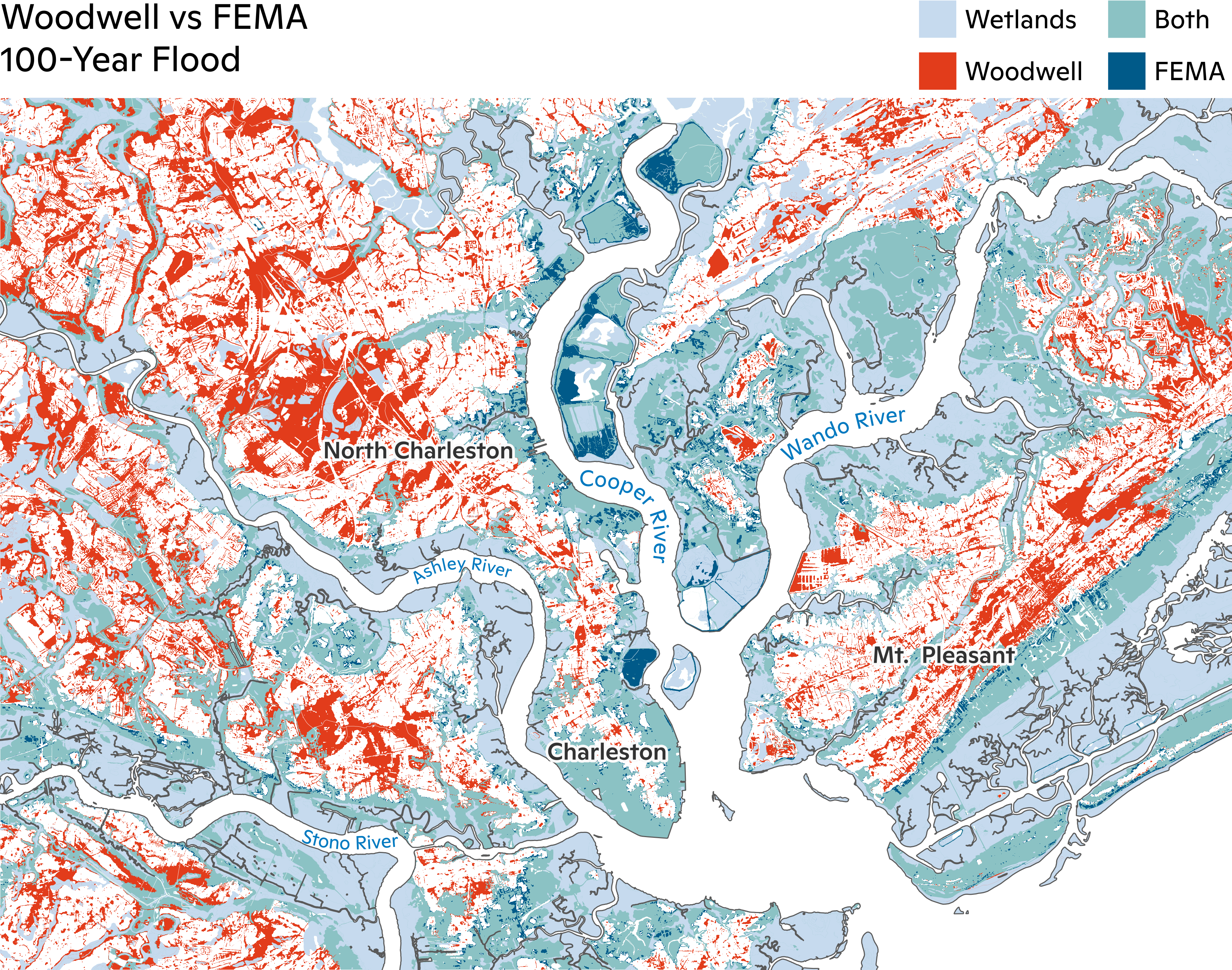
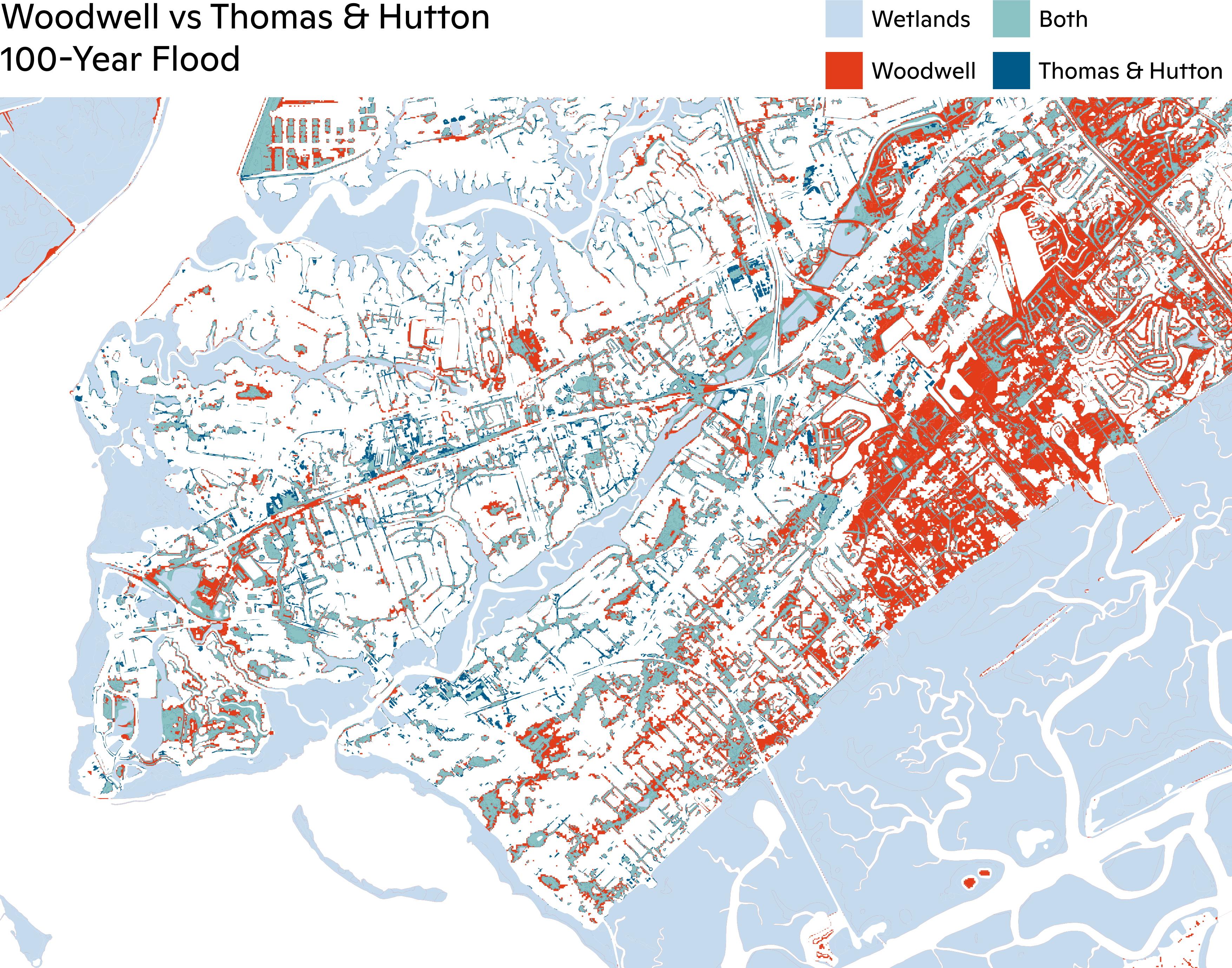
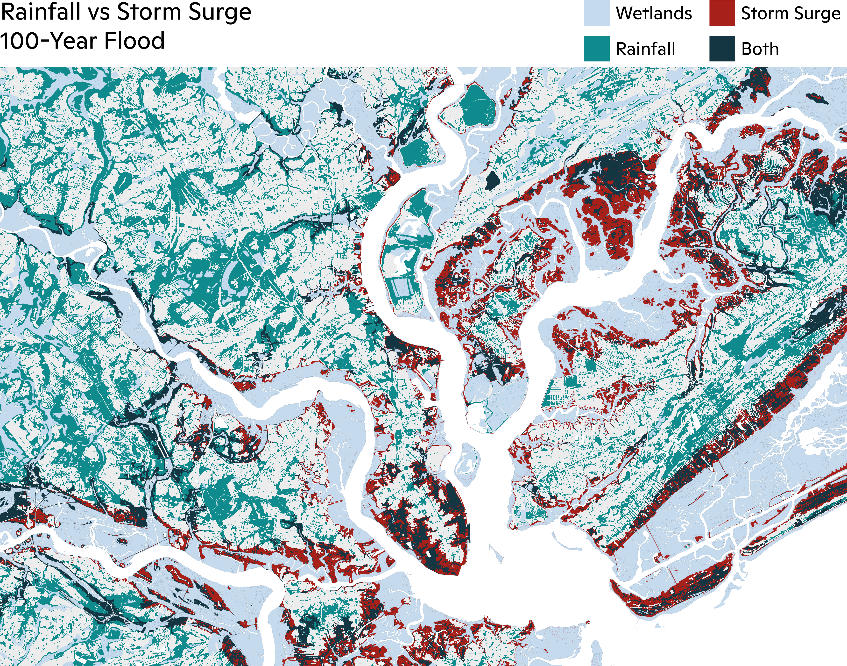
The county of Charleston is currently at high risk from flooding and this exposure will only increase under climate change. The results presented in this study were compared to FEMA’s flood maps, revealing significant discrepancies primarily due to the exclusion of pluvial flooding in FEMA’s analysis. A pluvial flood study conducted by Thomas & Hutton in Mount Pleasant was also used for comparison. The eastern side of the city exhibited substantial disagreements, likely attributable to differences in model setups.

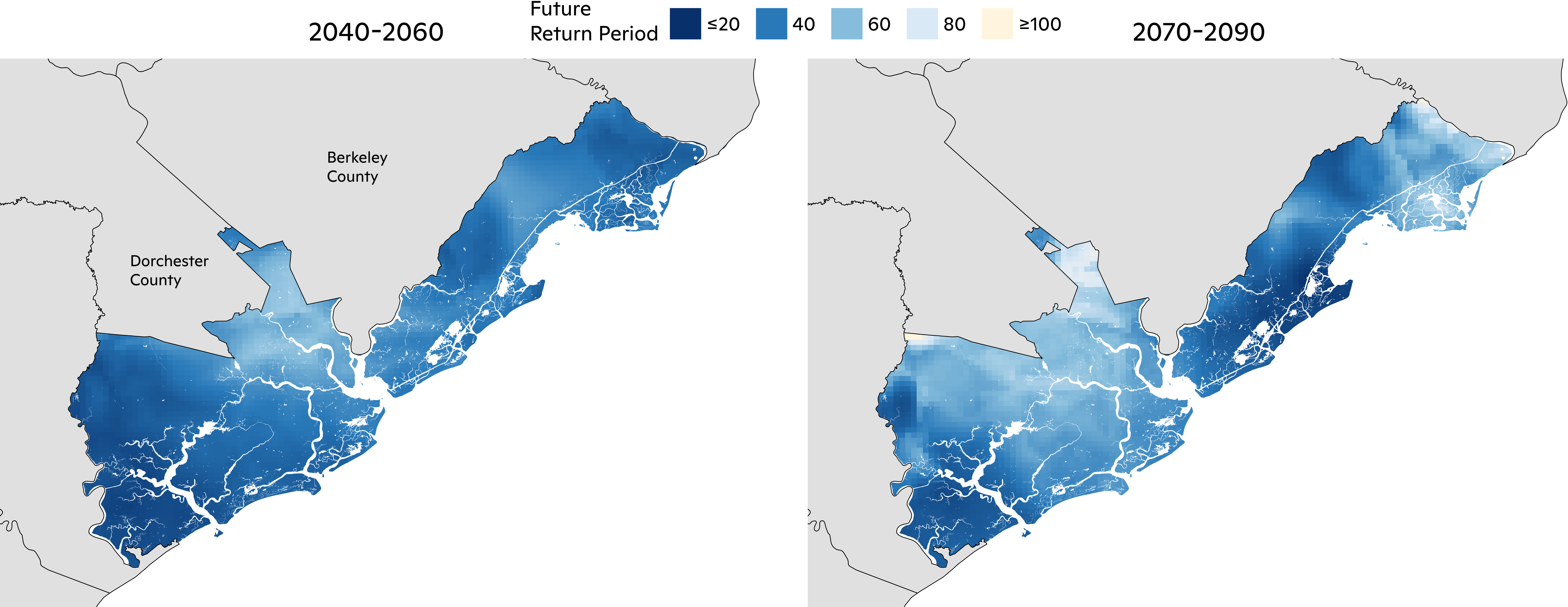
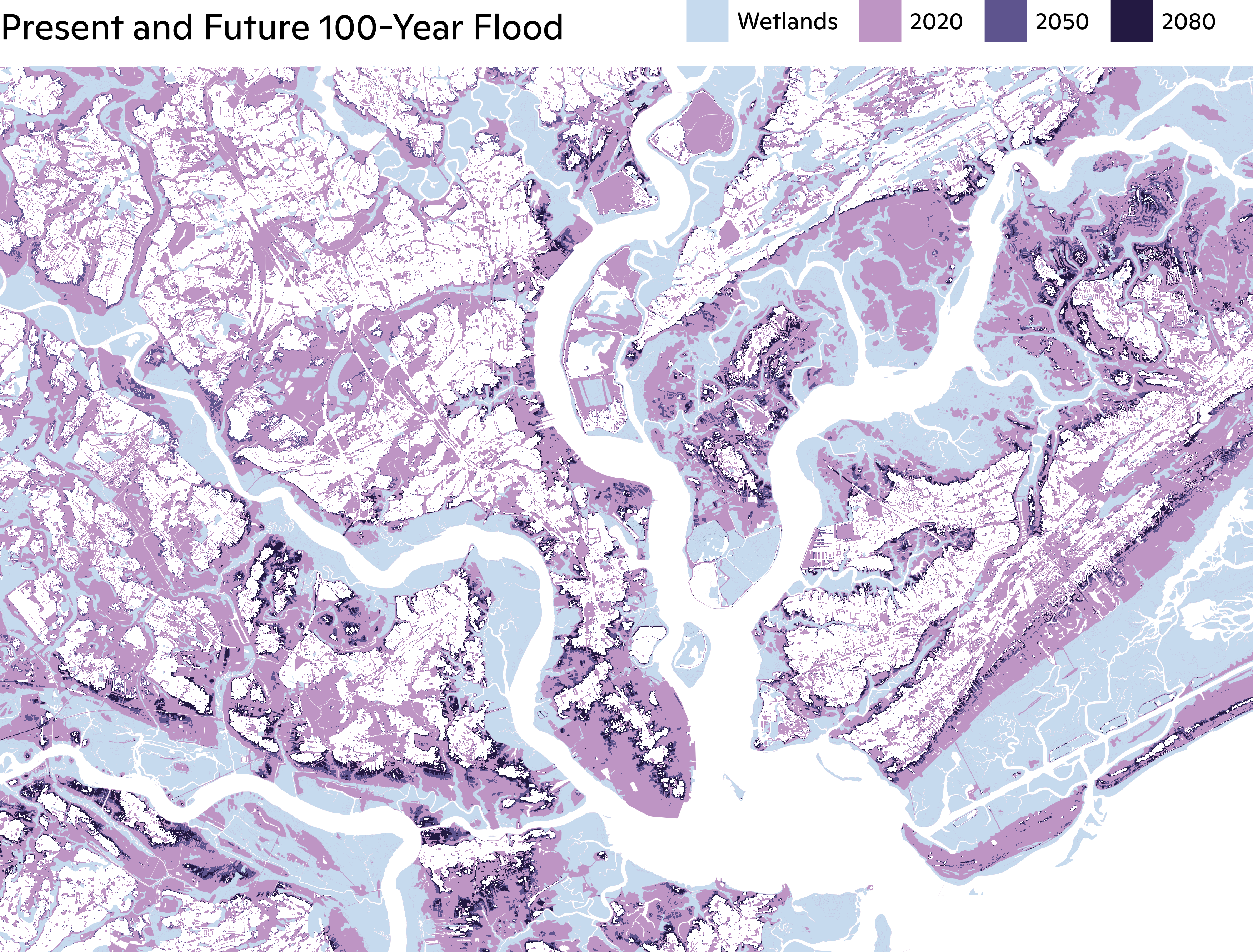
The results of this research indicate an expected increase in the frequency and intensity of heavy rainfall with the probability of the present-day 100-year rainfall event likely to triple by the mid 21st century and more than double (compared to present day) by the end of the century. Sea level rise is also an important contributor to changing flood risk for Charleston county. The projections from IPCC AR6 indicate significant sea level rise by 2050 (0.37 m) and 2080 (0.75 m) leading to larger flood extents. Given the scientific community’s limited knowledge on ice sheet dynamics, there is a nontrivial chance that an additional sea level rise of 1 to 2 feet on top of the SSP5-8.5 Low Confidence projection could occur by 2080. The aforementioned figures provide insight into the vulnerability of coastal and relatively inland areas, such as the downtown Charleston peninsula, North Charleston, and Mount Pleasant where an increasing number of buildings will be exposed to flood water by the end of the century.

Methodology

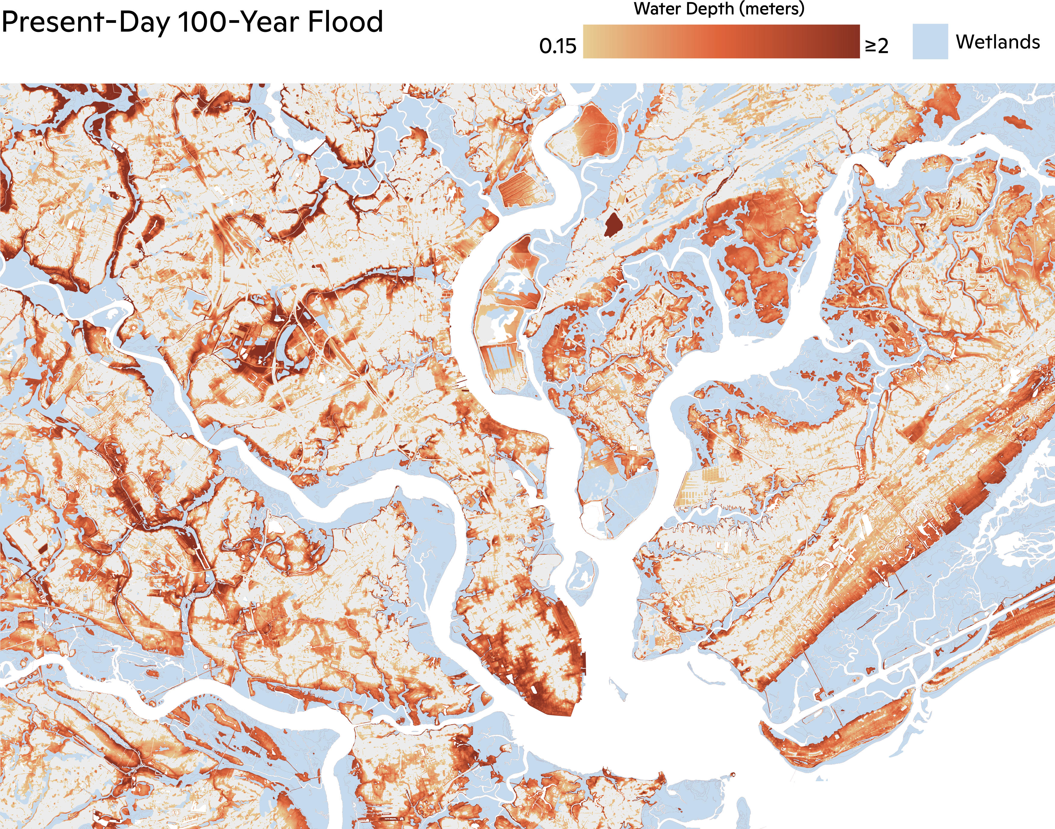
To simulate flood risk we use the LISFLOOD-FP v8.1 flood model (LISFLOOD-FP developers, 2022; Shaw et al., 2021). LISFLOOD-FP has been extensively used from the river reach scale to continental simulations and we refer the reader to Shaw et al. (2021) for a detailed explanation of LISFLOOD-FP. All flood model results show flooding above 15 cm as this is an average curb height and any flooding above this threshold would likely result in flood damages. All areas that are wetland and permanent water cover as determined by National Wetland Inventory (https://fwsprimary.wim.usgs.gov/wetlands/apps/wetlands-mapper). It should be noted that the western and eastern domain boundary results are not as robust as the rest of the domain because of the highly complex terrain and hydrology in the region.

Three time periods were used for this study: 2000–2020 (also referred to as present-day), 2040–2060, and 2070–2090. These time periods can also be interpreted as warming levels in the context of climate policy. The 2000–2020, 2040–2060, and 2070–2090 periods correspond to 1, 2 and 3 degrees Celsius of warming respectively. For each time period, a pluvial/riverine flooding run and a coastal flooding run were performed. We combine the two runs by taking the maximum depth for each pixel across the two model runs unless otherwise noted.

Any analysis involving structures used the USA Structures dataset (https://gis-fema.hub.arcgis.com/pages/usa-structures). This dataset was created through a collaboration between DHS, FIMA, FEMA’s Response Geospatial Office, Oak Ridge National Laboratory, and the U.S. Geological Survey.

1. RAINFALL
   A | Historical Rainfall
   The 24-hour 1-in-100 year rainfall event was used from NOAA Atlas 14 point precipitation frequency estimates for Charleston, SC (Bonnin et al., 2006). The temporal distribution, also from NOAA Atlas 14, of the 24 hour rainfall is taken from the combined cases of the four quartiles and uses the 90% cumulative probability.

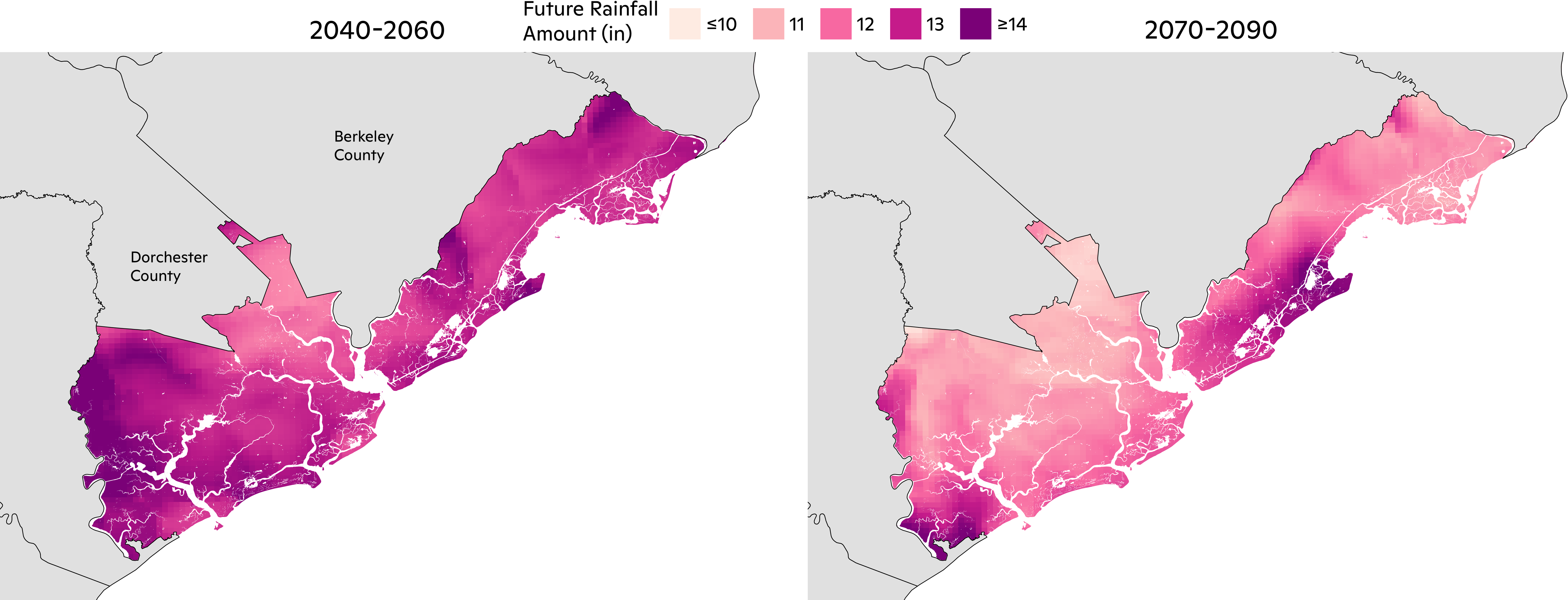
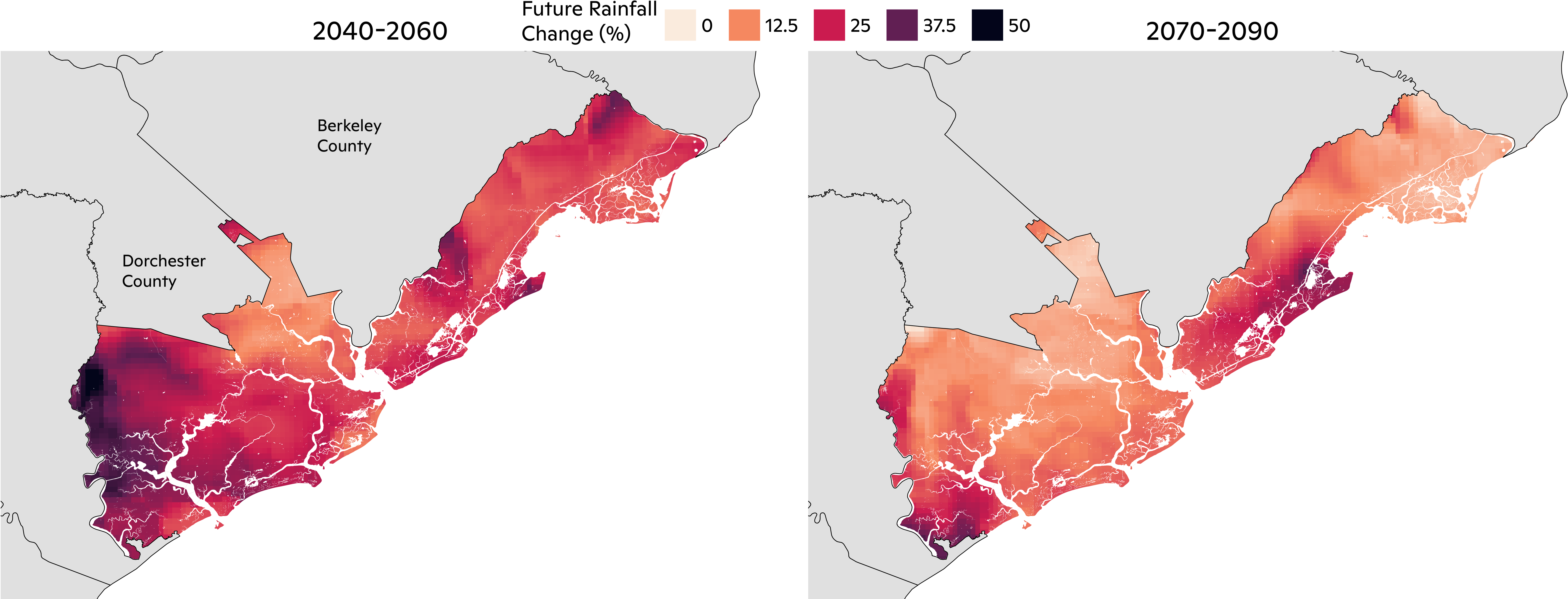
   B | Future Rainfall
   CMIP6 climate model data were bilinearly interpolated to a 1-km grid and then bias-adjusted using phase 3 of the Inter-Sectoral Impact Model Intercomparison Project (ISIMIP) version 2.5 methodology (ISIMIP3BASD v2.5) (Lange, 2019; Lange, 2021). High-resolution, 1-km Daymet reanalysis data (Thornton et al., 2022) were selected as the observation dataset for bias adjustment. Precipitation annual maxima were then extracted for three time periods, 2000–2020, 2040–2060, and 2070–2090 using the SSP5-8.5 scenario from the downscaled data. The annual maxima data for each pixel were fitted to a Generalized Extreme Value (GEV) distribution using the L-moments method (Hosking, 1990). The future return period of the historical (2000–2020) 1-in-100 year event is determined by finding the percentile in the future GEV distribution that corresponds with the historical rainfall amount. Rainfall amounts for the future 1-in-100 year events were estimated by determining what percentile in the historical period corresponds to the future 100-year amount, according to the future GEV. The percentile (analogous to a return period) was then converted to a rainfall amount using the rainfall distributions from the NOAA NA14 dataset.

2. DIGITAL ELEVATION MODEL
   For the majority of the Charleston County domain, the Continuously Updated Digital Elevation Model (CUDEM) from the NOAA National Centers for Environmental Information was used. The north western corner of the domain was not available, so it was included using the 2020 USGS Lidar DEM: Savannah Pee Dee, SC. The eastern edge of the DEM was also adjusted using the 2017 SC DNR Lidar DEM: Georgetown County, SC to fix a DEM boundary issue. The raw data from these sources was of variable resolution between 0.75m to 3m. The final DEM resolution was set to 10m due to the large model domain.
3. FRICTION COEFFICIENTS
   Friction coefficients, or Manning N values, were determined based on the land cover type of the area. The 2019 land cover was used for this from the National Land Cover Database (NLCD). Based on each classification of land cover, an associated friction coefficient is provided. See table here: https://rashms.com/wp-content/uploads/2021/01/Mannings-n-values-NLCD-NRCS.pdf
4. INFILTRATION
   To calculate soil infiltration rates, the USDA Soil Survey Geographic Database (SSURGO) for South Carolina was used to obtain the soil hydrologic groups. These hydrologic groups have defined infiltration rates depending on the type of soil. Infiltration values per hydrologic group were used from Musgrave (1955). These rates in combination with the NLCD impervious surface percentages were used to compute more accurate infiltration rates. The impervious surfaces take into account built-up areas where rainfall will not be able to infiltrate. We do not incorporate the impact of stormwater systems to convey runoff from streetscapes.
5. TIDE
   Tidal data was retrieved from the NOAA Tides and Currents. For Charleston, the mean higher high water, 0.8m and the mean lower low water, -0.957m were used. These values are relative to the vertical datum NAVD88.
6. STORM SURGE
   The FEMA flood insurance study reports were used to obtain 1-in-100 year storm surge values for points along the coast for Colleton, Charleston, and Georgetown counties. We do not account for shifting tropical cyclone distributions as this is beyond the scope of this study.
7. SEA LEVEL RISE
   Sea level rise data for Charleston, SC was taken from the IPCC AR6 Sea Level Projection Tool. We use the SSP5-8.5 Low Confidence scenario in order to maintain consistency with the future rainfall analysis. We use the low confidence scenario (which refers to greater Antarctica and Greenland ice sheet melting) because global sea level rise projections continue to increase as new data comes to light (Garner et al., 2018). Moreover, the scientific community’s understanding of Antarctica’s contribution to sea level rise is not strong enough to meaningfully differentiate between SSP5-8.5 and other scenarios except for SSP1-2.6 (van de Wal et al., 2022). However, there is only a 0.1% chance that society will experience the SSP1-2.6 scenario (Zeppetello et al., 2022). Additionally, the SSP5-8.5 Low Confidence scenario is roughly equivalent to the NOAA Intermediate scenario presented in the Interagency Sea Level Rise Scenario Tool.
8. STREAMFLOW
   We use the FEMA flood insurance study report to determine the streamflow entering the model domain. The available 1-in-100 year streamflow data that was the furthest upstream in the modeled domain was used. In this case, for the Edisto River along the county boundary of Colleton and Dorchester a 1-in-100 year value of 29,134 ft3/s. The Ashepoo River at US HWY 17 with a 1-in-100 year value of 7,990 ft3/s. Lastly, the Ashley River at US HWY 17A with a 1-in-100 year value of 10,070 ft3/s. All of these streamflow values are to account for water that would be moving downstream from rain falling outside of the model domain into the domain. We do not change streamflows for the future time periods as such hydrologic modeling is outside the scope of this study.
9. WATER DEPTH STARTFILE
   Due to the DEM containing bathymetry elevations in the Charleston Harbor and surrounding rivers, the model was initialized with starting water elevations representing a standard tide level. First, a permanent water mask was used to locate pixels that should be initialized with water elevations. Then, if the elevation of a pixel was less than the mean lower low water tide elevation, -0.957m NAVD88 in this case, then the starting water elevation for the pixel would be the tide level minus the DEM value.

Methodology references

Bonnin, G., Martin, D., Lin, B., Parzybok, T., Yekta, M., and Riley, D. (2004, rev. 2006). Precipitation-Frequency Atlas of the United States. Volume 2 Version 3.0: Delaware, District of Columbia, Illinois, Indiana, Kentucky, Maryland, New Jersey, North Carolina, Ohio, Pennsylvania, South Carolina, Tennessee, Virginia, West Virginia. NOAA Atlas 14. https://repository.library.noaa.gov/view/noaa/22610

Garner, A. J., Weiss, J. L., Parris, A., Kopp, R. E., Horton, R. M., Overpeck, J. T., and Horton, B. P. (2018). Evolution of 21st Century Sea Level Rise Projections. Earth’s Future 6(11), 1603-1615. https://doi.org/10.1029/2018EF000991

Hosking, J. R. (1990). L-moments: Analysis and Estimation of Distributions Using Linear Combinations of Order Statistics. Journal of the Royal Statistical Society: Series B (Methodological) 52(1), 105-124. https://www.jstor.org/stable/2345653

Lange, S. (2019). Trend-preserving Bias Adjustment and Statistical Downscaling with ISIMIP3BASD (v1. 0). Geoscientific Model Development 12(7), 3055-3070. https://doi.org/10.5194/gmd-12-3055-2019

Lange, Stefan. (2021). ISIMIP3BASD (2.5.0). Zenodo. https://doi.org/10.5281/zenodo.4686991
LISFLOOD-FP developers. (2022). LISFLOOD-FP 8.1 Hydrodynamic Model (8.1). Zenodo. https://doi.org/10.5281/zenodo.6912932

Musgrave, G. W. (1955). How Much of the Rain Enters the Soil? Yearbook of Agriculture 1955. https://naldc.nal.usda.gov/catalog/IND43894552

Shaw, J., Kesserwani, G., Neal, J., Bates, P., and Sharifian, M. K. (2021). LISFLOOD-FP 8.0:
The New Discontinuous Galerkin Shallow-water Solver for Multi-core CPUs and GPUs. Geoscientific Model Development 14(6), 3577-3602. https://doi.org/10.5194/gmd-14-3577-2021

Thornton, M.M., R. Shrestha, Y. Wei, P.E. Thornton, S-C. Kao, and B.E. Wilson. (2022). Daymet: Daily Surface Weather Data on a 1-km Grid for North America, Version 4 R1. ORNL DAAC, Oak Ridge, Tennessee, USA. https://doi.org/10.3334/ORNLDAAC/2129

van de Wal, R. S., Nicholls, R. J., Behar, D., McInnes, K., Stammer, D., Lowe, J. A., … and White, K. (2022). A High-End Estimate of Sea Level Rise for Practitioners. Earth’s Future 10(11). https://doi.org/10.1029/2022EF002751

Zeppetello, L. R. V., Raftery, A. E., and Battisti, D. S. (2022). Probabilistic Projections of Increased Heat Stress Driven by Climate Change. Communications Earth & Environment 3, 183. https://doi.org/10.1038/s43247-022-00524-4